Remote Sensing of Soil Organic Carbon (SOC)
- john06025
- Mar 20
- 5 min read
Updated: Mar 29
Soil organic carbon (SOC) is a key component of the global carbon cycle, and it plays a
vital role in the functioning of the terrestrial ecosystems. SOC levels are primarily
determined by photosynthesis (fixation of atmospheric CO2 into plant biomass),
respiration, and decomposition. The removal of atmospheric CO2, via photosynthesis,
is known as soil carbon sequestration. In the context of climate change, soil carbon
sequestration is emerging as an important tool for mitigating anthropogenic carbon
emissions [1].
Remote Sensing of SOC
Recent research has shown that SOC can be measured via a combination of satellite-
based remote sensing, and machine learning. Castaldi et al. [2] compared Sentinel-2
SOC predictions, with those from airborne hyperspectral data, using the following
methodology:
Three cloud-free S2 images were downloaded, with similar crop exposure conditions than during the airborne acquisitions.
Atmospherically correct for Bottom of Atmosphere (BOA) reflectance, using ESA SNAP.
Resample the atmospherically corrected images at 10m.
Select nine S2 bands: B2 (490nm), B3 (560nm), B4 (665nm), B5 (705nm), B6 (740nm), B7 (783nm), B8 (842nm), B11 (1610nm) and B12 (2190nm).
Mask everything that was not bare cropland soil at S2 acquisition time (bare soil pixels have NDVI <0.25).
Gather soil sample data: 2015 in Belgium (170 samples) and in 2016 in Luxembourg (194 samples), and in 2017 in Germany (231 samples). These locations were selected to encompass various SOC, and soil, types.
Measure ground truth SOC content for each soil sample (laboratory SOC).
Pair the ground truth SOC data with the S2, and airborne sensor, data, to thereby form the training dataset.
Two different multivariate models were tested for all spectral data: partial least square regression (PLSR) and random forest (RF). Prediction accuracy was evaluated using RMSE.
Each model was trained on matrices of the spectral bands (independent variables) and SOC content (dependent variable) using 10-folds cross validation
The authors found that the spatial resolution of Copernicus Sentinel-2 is adequate to
describe SOC variability both at field and regional scale, and the prediction accuracy
obtained by Copernicus Sentinel-2 data is similar to that retrieved by airborne
hyperspectral data. The most important spectral features for SOC prediction were
located in the VIS region at 450, 590 and 664nm, and very close to the S2 bands in
this spectral range (490, 560 and 665nm) [2].
![Figure 1. Soil organic carbon (SOC) maps of a field in Demmin area, obtained by HySpex (aerial) (a) and Sentinel-2 (b) data. Regional SOC is shown in the right figure [2].](https://static.wixstatic.com/media/86b4fe_f95c7b172c4c477e8a4c827f253d4001~mv2.png/v1/fill/w_980,h_618,al_c,q_90,usm_0.66_1.00_0.01,enc_avif,quality_auto/86b4fe_f95c7b172c4c477e8a4c827f253d4001~mv2.png)
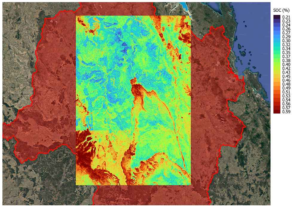
Geosynergy Proof of Concept for Fitzroy Basin
We demonstrated proof of concept remote sensing of SOC for the Fitzroy Basin region
of QLD. In the absence of field soil data samples, we used CSIRO data (Soil and
Landscape Grid National Soil Attribute Maps) [4]. There are maps (geotiffs) of bulk
density, SOC, clay, silt, sand, available water capacity, nitrogen, phosphorus, depth of
soil, depth of regolith, etc (at various depths).
Note that the CSIRO data is not field data, it is a combination of historical, and model-
generated, data. This is an important caveat, field soil data should be used for future
validation of the technique, before progressing to field use. Field samples should be
taken from the AOI, taken close to the time of Sentinel-2 sensing. Nonetheless, the
CSIRO data is sufficient to demonstrate POC.
A correlation matrix found that NTO and PTO were highly correlated to SOC, and
should therefore be excluded to avoid data leak. Other soil data features are less
highly correlated to SOC, and more readily available from soil maps, so can be used.

SOC was then modeled and predicted SOC for a large region of Fitzroy Basin (200 x
600 km), using CSIRO soil data and 6 Sentinel-2 products, as summarized in the
following figure:

Model accuracy was evaluated using per cell RMSE of the out of fold predictions. A
scatter plot of the predicted vs ground truth data is shown.

Lastly, the predicted SOC values were converted from CSV to Geotiff, allowing visual
display over the AOI, versus the ground truth CSIRO data.

Future Development
Again, it is important to remember that our POC is based on CSIRO soil data, which is
extrapolated from models. Modelling should be confirmed, and further developed,
using field samples. Note that sampling dates should be as close as possible to S2
sensing dates. The accuracy of the SOC maps is affected by the calibration dataset,
which should be representative of the investigated area while at the same time
including, as much as possible, the full range of SOC values [2].
Nonetheless, this POC, together with published accounts, such as those by Castaldi et
al. strongly indicate that this technique should be further developed for field use. The
fact that it is built on Sentinel-2 data, is also highly advantageous, due to its daily revisit time, global coverage, and open source availability.
The features used for modelling could be developed further. Regen Network, who are
active in this space, have discussed using other soil parameters, and geological
predictors, in their modelling including: clay composition %, silt composition %,
elevation (DEM), and topographic wetness index. They also stress that SOC is only
predicted to soil depth of the soil samples (with a target sampling depth of 10-15 cm)
[3].
The modeling approach could also be further developed. The Castaldi method only
uses 2 models (RF and PLSR), and there is considerable scope for testing model
ensembles (model stacking), as well as the use of deep networks. The current
approach extracts the soil / S2 data into tabular form, for modelling. However,
because of the data is inherently 2-dimensional, it would seem to be a natural fit for
approaches such as convolutional neural networks (CNNs).
References
[1] Soil Carbon Storage. Todd A. Ontl.
https://www.nature.com/scitable/knowledge/library/soil-carbon-storage-84223790/
[2] Castaldi, F., Hueni, A., Chabrillat, S., Ward, K., Buttafuoco, G., Bomans, B., Vreys,
K., Brell, M. and van Wesemael, B., 2019. Evaluating the capability of the Sentinel 2
data for soil organic carbon prediction in croplands. ISPRS Journal of Photogrammetry
and Remote Sensing, 147, pp.267-282.
[3] Regen Network, SOC remote sensing methodology.
https://app.regen.network/methodologies/carbonplus-grasslands
[4] CSIRO Soil and Landscape Grid National Soil Attribute Maps - Soil Organic Carbon
Fractions (3" resolution) - Release 1
Comments